Viz
Visualization of volumetric data.
qim3d.viz.chunks
Launches an interactive explorer for large-scale OME-Zarr and Zarr datasets.
This tool enables you to inspect massive 3D or 5D datasets (e.g., bio-imaging pyramids, large block-wise volumes) one chunk at a time without loading the entire file into RAM. It relies on lazy loading, making it ideal for checking data integrity, visualizing specific regions of interest (ROI) in big data, or navigating multi-resolution hierarchies.
Key Features:
- Lazy Exploration: Loads only the specific chunk selected via dropdown menus.
- Multiscale Support: Automatically detects and navigates resolution levels (pyramids) in OME-Zarr groups.
- 5D Navigation: Supports dimensions for Time (T) and Channel (C) in addition to spatial axes (Z, Y, X).
- Versatile Visualization: Switch instantly between a
slicer, aslices_grid, or a 3Dvolumetricrendering for the selected chunk.
Parameters:
| Name | Type | Description | Default |
|---|---|---|---|
zarr_path
|
str
|
The filesystem path to the OME-Zarr or Zarr dataset. |
required |
**kwargs
|
Any
|
Additional keyword arguments passed selectively to the underlying visualization function.
For example, you can pass |
{}
|
Returns:
| Name | Type | Description |
|---|---|---|
chunk_explorer |
VBox
|
The interactive interface containing controls for scale selection, chunk coordinates, and the visualization display. |
Raises:
| Type | Description |
|---|---|
ValueError
|
If the dataset dimensionality is not 3D or 5D. |
Example
Source code in qim3d/viz/_data_exploration.py
791 792 793 794 795 796 797 798 799 800 801 802 803 804 805 806 807 808 809 810 811 812 813 814 815 816 817 818 819 820 821 822 823 824 825 826 827 828 829 830 831 832 833 834 835 836 837 838 839 840 841 842 843 844 845 846 847 848 849 850 851 852 853 854 855 856 857 858 859 860 861 862 863 864 865 866 867 868 869 870 871 872 873 874 875 876 877 878 879 880 881 882 883 884 885 886 887 888 889 890 891 892 893 894 895 896 897 898 899 900 901 902 903 904 905 906 907 908 909 910 911 912 913 914 915 916 917 918 919 920 921 922 923 924 925 926 927 928 929 930 931 932 933 934 935 936 937 938 939 940 941 942 943 944 945 946 947 948 949 950 951 952 953 954 955 956 957 958 959 960 961 962 963 964 965 966 967 968 969 970 971 972 973 974 975 976 977 978 979 980 981 982 983 984 985 986 987 988 989 990 991 992 993 994 995 996 997 998 999 1000 1001 1002 1003 1004 1005 1006 1007 1008 1009 1010 1011 | |
qim3d.viz.circles
Visualizes detected blobs as circles overlaid on the volume slices.
This function is primarily used to verify the results of blob detection algorithms. It takes a list of detected features (defined by their center coordinates and radius) and projects them onto the 2D slices of the volume. As you scroll through the stack, the circles dynamically resize to represent the cross-section of the 3D spherical blobs at that specific depth, providing an intuitive check for detection accuracy.
Parameters:
| Name | Type | Description | Default |
|---|---|---|---|
blobs
|
ndarray
|
A list or array of detected blobs. Each blob is expected to be a 4-tuple or array |
required |
volume
|
ndarray
|
The 3D volume (image stack) on which the blobs were detected. |
required |
alpha
|
float
|
The transparency level of the filled circles (0.0 to 1.0). Defaults to 0.5. |
0.5
|
color
|
str
|
The color of the circles, capable of accepting hex codes or standard color names. Defaults to "#ff9900" (orange). |
'#ff9900'
|
**kwargs
|
Any
|
Additional keyword arguments passed to the underlying |
{}
|
Returns:
| Name | Type | Description |
|---|---|---|
slicer_obj |
interactive
|
An interactive widget with a slider to navigate through slices, showing the overlay of detected blobs. |
Example
import qim3d
import qim3d.detection

# Get data
vol = qim3d.examples.cement_128x128x128

# Detect blobs, and get binary mask
blobs, _ = qim3d.detection.blobs(
    vol,
    min_sigma=1,
    max_sigma=8,
    threshold=0.001,
    overlap=0.1,
    background="bright"
    )

# Visualize detected blobs with circles method
qim3d.viz.circles(blobs, vol, alpha=0.8, color='blue')
Source code in qim3d/viz/_detection.py
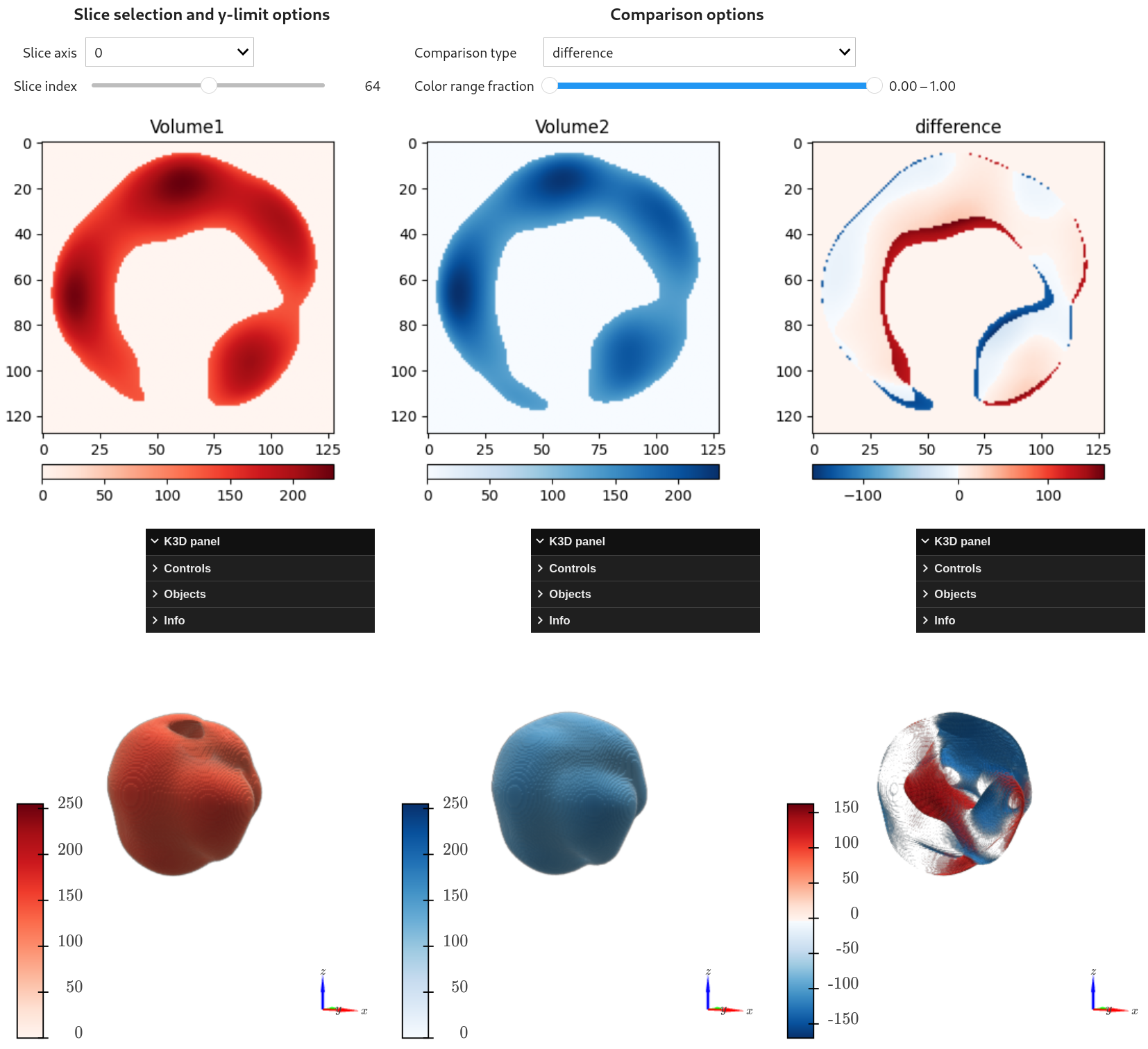
qim3d.viz.compare_volumes
Launches an interactive dashboard to visually compare two 3D volumes side-by-side.
This tool is essential for registration validation (checking alignment), change detection, or analyzing reconstruction errors (residuals). It displays synchronized slices of both volumes alongside a computed difference map. You can switch between 'difference', 'absolute difference', and 'quadratic difference' modes to highlight discrepancies effectively.
If enabled, the tool also provides 3D volumetric rendering (via k3d), allowing you to inspect the spatial distribution of the errors or changes in 3D space.
Parameters:
| Name | Type | Description | Default |
|---|---|---|---|
volume1
|
ndarray
|
The first 3D volume (e.g., Ground Truth or Reference). |
required |
volume2
|
ndarray
|
The second 3D volume (e.g., Prediction or Moving Image). Must have the same shape as |
required |
slice_axis
|
int
|
The initial axis along which to slice (0, 1, or 2). Defaults to 0. |
0
|
slice_index
|
int
|
The initial slice index to display. If |
None
|
volumetric_visualization
|
bool
|
If |
False
|
Returns:
| Name | Type | Description |
|---|---|---|
widget |
VBox
|
The interactive widget containing the comparison controls, slice plots, and optional 3D views. |
Example
import qim3d
vol1 = qim3d.generate.volume(noise_scale=0.020, dtype='float32')
vol2 = qim3d.generate.volume(noise_scale=0.021, dtype='float32')
qim3d.viz.compare_volumes(vol1, vol2, volumetric_visualization=True)
Source code in qim3d/viz/_data_exploration.py
2208 2209 2210 2211 2212 2213 2214 2215 2216 2217 2218 2219 2220 2221 2222 2223 2224 2225 2226 2227 2228 2229 2230 2231 2232 2233 2234 2235 2236 2237 2238 2239 2240 2241 2242 2243 2244 2245 2246 2247 2248 2249 2250 2251 2252 2253 2254 2255 2256 2257 2258 2259 2260 2261 2262 2263 2264 2265 2266 2267 2268 2269 2270 2271 2272 2273 | |
qim3d.viz.export_rotation
export_rotation(path, volume, degrees=360, n_frames=180, fps=30, image_size=(256, 256), colormap='magma', camera_height=2.0, camera_distance='auto', camera_focus='center', show=False)
Exports a 360-degree turntable animation of the volume to a video or GIF.
Generates a spinning orbit visualization of the 3D data, perfect for presentations, reports, or sharing results on the web. It renders the volume from a rotating camera perspective and saves the output as a movie file (.mp4, .webm, .avi) or an animated .gif.
Key Features:
- Presentation Ready: Creates smooth, professional animations of your data.
- Flexible Output: Supports common video formats and high-quality GIFs.
- Customizable Camera: Control the height, distance, and focus point of the rotation.
Parameters:
| Name | Type | Description | Default |
|---|---|---|---|
path
|
str
|
The destination file path. Must end with .gif, .avi, .mp4, or .webm. If no extension is provided, defaults to .gif. |
required |
volume
|
ndarray
|
The 3D input volume to be animated. |
required |
degrees
|
int
|
Total rotation angle in degrees (e.g., 360 for a full spin). |
360
|
n_frames
|
int
|
Total number of frames to generate. Higher values create smoother/slower animations at fixed FPS. |
180
|
fps
|
int
|
Frames per second. Controls the playback speed. |
30
|
image_size
|
tuple[int, int] or None
|
Resolution (width, height) of the output frames. |
(256, 256)
|
colormap
|
str
|
Matplotlib colormap name for the volume rendering. |
'magma'
|
camera_height
|
float
|
Vertical position of the camera relative to the volume's Z-axis height. |
2.0
|
camera_distance
|
float or str
|
Distance from the camera to the focus point.
|
'auto'
|
camera_focus
|
list or str
|
The point the camera rotates around.
|
'center'
|
show
|
bool
|
If |
False
|
Raises:
| Type | Description |
|---|---|
TypeError
|
If |
ValueError
|
If |
Example
Creation of .gif file with default parameters of a generated volume.
Example
Creation of a .webm file with specified parameters of a generated volume in the shape of a tube.
import qim3d
vol = qim3d.generate.volume(shape='tube')
qim3d.viz.export_rotation('test.webm', vol,
degrees = 360,
n_frames = 120,
fps = 30,
image_size = (512,512),
camera_height = 3.0,
camera_distance = 'auto',
camera_focus = 'center',
show = True)
Source code in qim3d/viz/_data_exploration.py
2522 2523 2524 2525 2526 2527 2528 2529 2530 2531 2532 2533 2534 2535 2536 2537 2538 2539 2540 2541 2542 2543 2544 2545 2546 2547 2548 2549 2550 2551 2552 2553 2554 2555 2556 2557 2558 2559 2560 2561 2562 2563 2564 2565 2566 2567 2568 2569 2570 2571 2572 2573 2574 2575 2576 2577 2578 2579 2580 2581 2582 2583 2584 2585 2586 2587 2588 2589 2590 2591 2592 2593 2594 2595 2596 2597 2598 2599 2600 2601 2602 2603 2604 2605 2606 2607 2608 2609 2610 2611 2612 2613 2614 2615 2616 2617 2618 2619 2620 2621 2622 2623 2624 2625 2626 2627 2628 2629 2630 2631 2632 2633 2634 2635 2636 2637 2638 2639 2640 2641 2642 2643 2644 2645 2646 2647 2648 2649 2650 2651 2652 2653 2654 2655 2656 2657 2658 2659 2660 2661 2662 2663 2664 2665 2666 2667 2668 2669 2670 2671 2672 2673 2674 2675 2676 2677 2678 2679 2680 2681 2682 2683 2684 2685 2686 2687 2688 2689 2690 2691 2692 2693 2694 2695 2696 2697 | |
qim3d.viz.fade_mask
Launches an interactive tool to tune parameters for edge fading (vignetting) on a 3D volume.
This function helps you find the optimal settings for suppressing boundary artifacts or focusing on the center of the volume. It visualizes the process by displaying three panels: the original slice, the generated weight mask (attenuation map), and the final result. You can adjust the decay rate, ratio (radius), and geometry (spherical or cylindrical) in real-time before applying them permanently using qim3d.operations.fade_mask.
Parameters:
| Name | Type | Description | Default |
|---|---|---|---|
volume
|
ndarray
|
The 3D input volume. |
required |
axis
|
int
|
The axis alignment for the mask geometry (relevant for cylindrical fading). Defaults to 0. |
0
|
colormap
|
str
|
The Matplotlib colormap used for displaying the volume and mask. Defaults to 'magma'. |
'magma'
|
min_value
|
float
|
Custom minimum intensity for display contrast. If |
None
|
max_value
|
float
|
Custom maximum intensity for display contrast. If |
None
|
Returns:
| Name | Type | Description |
|---|---|---|
slicer_obj |
interactive
|
The interactive widget containing the parameter sliders and the side-by-side visualization. |
Source code in qim3d/viz/_data_exploration.py
638 639 640 641 642 643 644 645 646 647 648 649 650 651 652 653 654 655 656 657 658 659 660 661 662 663 664 665 666 667 668 669 670 671 672 673 674 675 676 677 678 679 680 681 682 683 684 685 686 687 688 689 690 691 692 693 694 695 696 697 698 699 700 701 702 703 704 705 706 707 708 709 710 711 712 713 714 715 716 717 718 719 720 721 722 723 724 725 726 727 728 729 730 731 732 733 734 735 736 737 738 739 740 741 742 743 744 745 746 747 748 749 750 751 752 753 754 755 756 757 758 759 760 761 762 763 764 765 766 767 768 769 770 771 772 773 774 775 776 777 778 779 780 781 782 783 784 785 786 787 788 | |
qim3d.viz.grid_overview
Displays an overview grid of images, labels, and masks (if they exist).
Labels are the annotated target segmentations Masks are applied to the output and target prior to the loss calculation in case of sparse labeled data
Parameters:
| Name | Type | Description | Default |
|---|---|---|---|
data
|
list or Dataset
|
A list of tuples or Torch dataset containing image, label, (and mask data). |
required |
n_images
|
int
|
The maximum number of images to display. Defaults to 7. |
7
|
colormap_im
|
str
|
The colormap to be used for displaying input images. Defaults to 'gray'. |
'gray'
|
colormap_segm
|
str
|
The colormap to be used for displaying labels. Defaults to 'viridis'. |
'viridis'
|
alpha
|
float
|
The transparency level of the label and mask overlays. Defaults to 0.5. |
0.5
|
show
|
bool
|
If True, displays the plot (i.e. calls plt.show()). Defaults to False. |
False
|
Raises:
| Type | Description |
|---|---|
ValueError
|
If the data elements are not tuples. |
Returns:
| Name | Type | Description |
|---|---|---|
fig |
Figure
|
The figure with an overview of the images and their labels. |
Notes
- If the image data is RGB, the color map is ignored and the user is informed.
- The number of displayed images is limited to the minimum between
n_imagesand the length of the data. - The grid layout and dimensions vary based on the presence of a mask.
Source code in qim3d/viz/_metrics.py
85 86 87 88 89 90 91 92 93 94 95 96 97 98 99 100 101 102 103 104 105 106 107 108 109 110 111 112 113 114 115 116 117 118 119 120 121 122 123 124 125 126 127 128 129 130 131 132 133 134 135 136 137 138 139 140 141 142 143 144 145 146 147 148 149 150 151 152 153 154 155 156 157 158 159 160 161 162 163 164 165 166 167 168 169 170 171 172 173 174 175 176 177 178 | |
qim3d.viz.grid_pred
grid_pred(in_targ_preds, n_images=7, colormap_im='gray', colormap_segm='viridis', alpha=0.5, show=False)
Displays a grid of input images, predicted segmentations, ground truth segmentations, and their comparison.
Displays a grid of subplots representing different aspects of the input images and segmentations. The grid includes the following rows: - Row 1: Input images - Row 2: Predicted segmentations overlaying input images - Row 3: Ground truth segmentations overlaying input images - Row 4: Comparison between true and predicted segmentations overlaying input images
Each row consists of n_images subplots, where each subplot corresponds to an image from the dataset.
The function utilizes various color maps for visualization and applies transparency to the segmentations.
Parameters:
| Name | Type | Description | Default |
|---|---|---|---|
in_targ_preds
|
tuple
|
A tuple containing input images, target segmentations, and predicted segmentations. |
required |
n_images
|
int
|
Number of images to display. Defaults to 7. |
7
|
colormap_im
|
str
|
Color map for input images. Defaults to "gray". |
'gray'
|
colormap_segm
|
str
|
Color map for segmentations. Defaults to "viridis". |
'viridis'
|
alpha
|
float
|
Alpha value for transparency. Defaults to 0.5. |
0.5
|
show
|
bool
|
If True, displays the plot (i.e. calls plt.show()). Defaults to False. |
False
|
Returns:
| Name | Type | Description |
|---|---|---|
fig |
Figure
|
The figure with images, labels and the label prediction from the trained models. |
Example
import qim3d dataset = MySegmentationDataset() model = MySegmentationModel() in_targ_preds = qim3d.ml.inference(dataset,model) qim3d.viz.grid_pred(in_targ_preds, colormap_im='viridis', alpha=0.5)
Source code in qim3d/viz/_metrics.py
181 182 183 184 185 186 187 188 189 190 191 192 193 194 195 196 197 198 199 200 201 202 203 204 205 206 207 208 209 210 211 212 213 214 215 216 217 218 219 220 221 222 223 224 225 226 227 228 229 230 231 232 233 234 235 236 237 238 239 240 241 242 243 244 245 246 247 248 249 250 251 252 253 254 255 256 257 258 259 260 261 262 263 264 265 266 267 268 269 270 271 272 273 274 275 276 277 278 279 280 281 282 283 284 285 286 287 288 289 290 | |
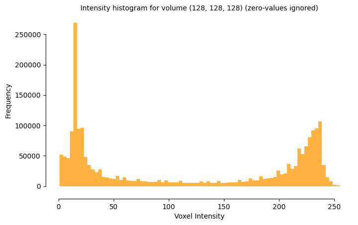
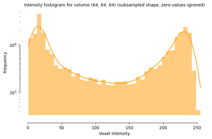
qim3d.viz.histogram
histogram(volume, coarseness=1, ignore_zero=True, bins='auto', slice_index=None, slice_axis=0, vertical_line=None, vertical_line_colormap='qim', kde=False, log_scale=False, despine=True, show_title=True, color='qim3d', edgecolor=None, figsize=(8, 4.5), bin_style='step', return_fig=False, show=True, ax=None, **sns_kwargs)
Computes and displays the intensity distribution (histogram) of a 3D volume or a specific 2D slice.
This function visualizes the frequency of voxel intensities (gray values), which is essential for analyzing data contrast, identifying material phases, and determining threshold values for segmentation. It utilizes seaborn.histplot and includes optimizations for 3D data, such as subsampling (coarseness) to handle large datasets efficiently. You can also overlay Kernel Density Estimates (KDE) or specific threshold markers.
Parameters:
| Name | Type | Description | Default |
|---|---|---|---|
volume
|
ndarray
|
The 3D input volume. |
required |
coarseness
|
int or list[int]
|
Subsampling factor to speed up computation. A value of |
1
|
ignore_zero
|
bool
|
If |
True
|
bins
|
int or str
|
The number of bins or a binning strategy (e.g., 'auto', 'sturges'). |
'auto'
|
slice_index
|
int, str, or None
|
The specific slice to analyze. If |
None
|
slice_axis
|
int
|
The axis along which to extract the slice (0, 1, or 2). Used only if |
0
|
vertical_line
|
int or Iterable
|
One or more intensity values to mark with vertical dashed lines (e.g., to visualize a threshold cut-off). |
None
|
vertical_line_colormap
|
str or Iterable
|
The colormap or list of colors for the vertical lines. |
'qim'
|
kde
|
bool
|
If |
False
|
log_scale
|
bool
|
If |
False
|
despine
|
bool
|
If |
True
|
show_title
|
bool
|
If |
True
|
color
|
str
|
The main color of the histogram bars. |
'qim3d'
|
edgecolor
|
str
|
The color of the bar edges. |
None
|
figsize
|
tuple[float, float]
|
The width and height of the figure in inches. |
(8, 4.5)
|
bin_style
|
str
|
The visual style of the histogram ('bars', 'step', or 'poly'). |
'step'
|
return_fig
|
bool
|
If |
False
|
show
|
bool
|
If |
True
|
ax
|
Axes
|
An existing Axes object to plot onto. If provided, the function returns this Axes object (unless |
None
|
**sns_kwargs
|
str | float | bool
|
Additional keyword arguments passed to |
{}
|
Returns:
| Name | Type | Description |
|---|---|---|
object |
matplotlib.figure.Figure, matplotlib.axes.Axes, or None
|
The plot object, depending on parameters:
|
Raises:
| Type | Description |
|---|---|
ValueError
|
If |
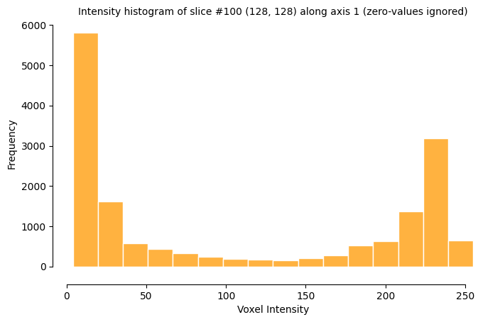
Histogram from a single slice
import qim3d
vol = qim3d.examples.bone_128x128x128
qim3d.viz.histogram(vol, slice_index=100, slice_axis=1, bin_style='bars', edgecolor='white')
Using coarseness for faster computation
import qim3d
vol = qim3d.examples.bone_128x128x128
qim3d.viz.histogram(vol, coarseness=2, kde=True, log_scale=True)
Source code in qim3d/viz/_data_exploration.py
1014 1015 1016 1017 1018 1019 1020 1021 1022 1023 1024 1025 1026 1027 1028 1029 1030 1031 1032 1033 1034 1035 1036 1037 1038 1039 1040 1041 1042 1043 1044 1045 1046 1047 1048 1049 1050 1051 1052 1053 1054 1055 1056 1057 1058 1059 1060 1061 1062 1063 1064 1065 1066 1067 1068 1069 1070 1071 1072 1073 1074 1075 1076 1077 1078 1079 1080 1081 1082 1083 1084 1085 1086 1087 1088 1089 1090 1091 1092 1093 1094 1095 1096 1097 1098 1099 1100 1101 1102 1103 1104 1105 1106 1107 1108 1109 1110 1111 1112 1113 1114 1115 1116 1117 1118 1119 1120 1121 1122 1123 1124 1125 1126 1127 1128 1129 1130 1131 1132 1133 1134 1135 1136 1137 1138 1139 1140 1141 1142 1143 1144 1145 1146 1147 1148 1149 1150 1151 1152 1153 1154 1155 1156 1157 1158 1159 1160 1161 1162 1163 1164 1165 1166 1167 1168 1169 1170 1171 1172 1173 1174 1175 1176 1177 1178 1179 1180 1181 1182 1183 1184 1185 1186 1187 1188 1189 1190 1191 1192 1193 1194 1195 1196 1197 1198 1199 1200 1201 1202 1203 1204 | |
qim3d.viz.image_preview
Image preview function
Source code in qim3d/viz/_preview.py
qim3d.viz.iso_surface
Creates an interactive tool to visualize 3D iso-surfaces (surfaces of constant value).
Generates a GUI to extract and render 3D contours from the volume in real-time. This is useful for finding specific intensity boundaries, visualizing segmentation masks, or exploring the shape of objects defined by a specific threshold. It uses Plotly for interaction and includes controls for resolution and transparency.
Key Features:
- Interactive Thresholding: Adjust the iso-value dynamically to see how the surface changes.
- Performance Control: Adjustable resolution slider to balance between mesh quality and rendering speed.
- Visual Styles: Supports wireframe mode, transparency, and various colormaps.
Parameters:
| Name | Type | Description | Default |
|---|---|---|---|
volume
|
ndarray
|
The 3D input volume to be visualized. |
required |
colormap
|
str
|
The initial color map name (e.g., 'Magma', 'Viridis'). Can be changed in the GUI. |
'Magma'
|
Source code in qim3d/viz/_data_exploration.py
qim3d.viz.line_profile
line_profile(volume, slice_axis=0, slice_index='middle', vertical_position='middle', horizontal_position='middle', angle=0, fraction_range=(0.0, 1.0), y_limits='auto')
Creates an interactive tool to visualize intensity profiles along a line segment within a 3D volume.
This function allows you to draw a line on a specific slice of your data and plot the pixel or voxel intensity values along that path. It is ideal for quantitative analysis, such as checking material homogeneity, measuring the sharpness of edges (step functions), or inspecting noise levels across a region of interest (ROI). The tool supports arbitrary angles, dynamic pivot points, and adjustable plot limits.
Key Features:
- Profile Plotting: Real-time graph of intensity values (gray levels) versus distance.
- Flexible Positioning: Define the line by a pivot point (vertical/horizontal) and an angle of rotation.
- Navigation: Select specific slices using indices or keywords like 'middle'.
- Zooming: Focus on specific segments of the line using the
fraction_rangeparameter.
Parameters:
| Name | Type | Description | Default |
|---|---|---|---|
volume
|
ndarray
|
The 3D input volume (image stack). |
required |
slice_axis
|
int
|
The axis along which to extract the 2D slice (0, 1, or 2). Defaults to 0. |
0
|
slice_index
|
int or str
|
The index of the slice to display. Can be an integer or a position string ('start', 'middle', 'end'). Defaults to 'middle'. |
'middle'
|
vertical_position
|
int or str
|
The vertical coordinate of the line's pivot point. Can be an integer or 'start', 'middle', 'end'. Defaults to 'middle'. |
'middle'
|
horizontal_position
|
int or str
|
The horizontal coordinate of the line's pivot point. Can be an integer or 'start', 'middle', 'end'. Defaults to 'middle'. |
'middle'
|
angle
|
int or float
|
The angle of the line in degrees relative to the horizontal axis. Floats are rounded to the nearest integer. Defaults to 0. |
0
|
fraction_range
|
tuple[float, float]
|
The start and end points of the line segment as a fraction of the image width/height (0.0 to 1.0). Defaults to (0.00, 1.00). |
(0.0, 1.0)
|
y_limits
|
str or tuple[float, float]
|
Controls the Y-axis range of the intensity plot. Defaults to 'auto'.
|
'auto'
|
Returns:
| Name | Type | Description |
|---|---|---|
widget |
interactive
|
The interactive widget object containing the slice viewer and the intensity plot. |
Source code in qim3d/viz/_data_exploration.py
1481 1482 1483 1484 1485 1486 1487 1488 1489 1490 1491 1492 1493 1494 1495 1496 1497 1498 1499 1500 1501 1502 1503 1504 1505 1506 1507 1508 1509 1510 1511 1512 1513 1514 1515 1516 1517 1518 1519 1520 1521 1522 1523 1524 1525 1526 1527 1528 1529 1530 1531 1532 1533 1534 1535 1536 1537 1538 1539 1540 1541 1542 1543 1544 1545 1546 1547 1548 1549 1550 1551 1552 1553 1554 1555 1556 1557 1558 1559 1560 1561 1562 1563 1564 1565 1566 1567 1568 1569 1570 1571 1572 1573 1574 1575 1576 1577 1578 1579 1580 1581 1582 1583 1584 1585 1586 1587 1588 1589 1590 1591 1592 1593 1594 1595 1596 1597 1598 1599 1600 1601 1602 1603 1604 1605 1606 1607 1608 1609 1610 1611 | |
qim3d.viz.local_thickness
local_thickness(image, image_lt, max_projection=False, axis=0, slice_index=None, show=False, figsize=(15, 5))
Visualizes a local thickness map alongside the original image and a statistics histogram.
This function provides a comprehensive view of structure width or pore size distribution. It displays a side-by-side comparison of the original data and the computed local thickness (heat map), where color intensity represents the diameter of the largest sphere that fits inside the structure at that point. It also includes a histogram to quantify the distribution of thickness values.
For 3D volumes, the output can be either an interactive slice viewer or a static Maximum Intensity Projection (MIP).
Parameters:
| Name | Type | Description | Default |
|---|---|---|---|
image
|
ndarray
|
The original 2D or 3D input data (binary or grayscale). |
required |
image_lt
|
ndarray
|
The computed local thickness map (must have the same shape as |
required |
max_projection
|
bool
|
If |
False
|
axis
|
int
|
The axis along which to slice or project the volume. Defaults to 0. |
0
|
slice_index
|
int or float
|
The initial slice to display for 3D volumes.
|
None
|
show
|
bool
|
If |
False
|
figsize
|
tuple[int, int]
|
The width and height of the figure in inches. Defaults to (15, 5). |
(15, 5)
|
Returns:
| Name | Type | Description |
|---|---|---|
object |
interactive or Figure
|
The visualization object, depending on the input and parameters:
|
Raises:
| Type | Description |
|---|---|
ValueError
|
If |
Example
import qim3d
fly = qim3d.examples.fly_150x256x256
lt_fly = qim3d.processing.local_thickness(fly)
qim3d.viz.local_thickness(fly, lt_fly, axis=0)
Source code in qim3d/viz/_local_thickness.py
10 11 12 13 14 15 16 17 18 19 20 21 22 23 24 25 26 27 28 29 30 31 32 33 34 35 36 37 38 39 40 41 42 43 44 45 46 47 48 49 50 51 52 53 54 55 56 57 58 59 60 61 62 63 64 65 66 67 68 69 70 71 72 73 74 75 76 77 78 79 80 81 82 83 84 85 86 87 88 89 90 91 92 93 94 95 96 97 98 99 100 101 102 103 104 105 106 107 108 109 110 111 112 113 114 115 116 117 118 119 120 121 122 123 124 125 126 127 128 129 130 131 132 133 134 135 136 137 138 139 | |
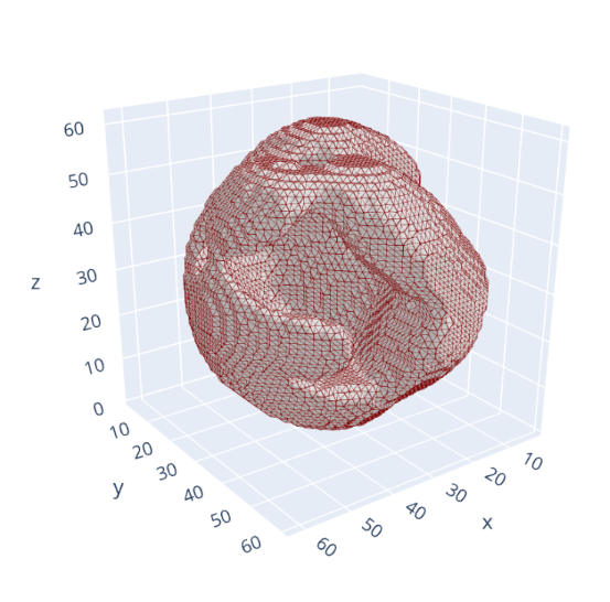
qim3d.viz.mesh
mesh(mesh, wireframe=False, show_edges=True, show=True, save_screenshot='', export_html='', explode=0, smooth_shading=False, face_color='#cccccc', edge_color='#993333', **kwargs)
Visualize a 3D mesh using pygel3d or pyvista. If you need more advanced tools, use pyvista directly.
Parameters:
| Name | Type | Description | Default |
|---|---|---|---|
mesh
|
Manifold
|
The input mesh object. |
required |
wireframe
|
bool
|
If True, displays the mesh as a wireframe. Defaults to False. |
False
|
show_edges
|
bool
|
If True, shows edges of the mesh. Fefaults to True. |
True
|
show
|
bool
|
If True, displays the visualization inline, useful for multiple plots.
Works only with backend |
True
|
save_screenshot
|
str
|
If True, saves the visualization as an |
''
|
export_html
|
str
|
If True, saves the visualization as an |
''
|
explode
|
int
|
Only works when mesh is qim3d.mesh.VolumeMesh. Defines how spread are the tetrahedrons. If 0, the volume us intact. Defaults to 1. |
0
|
smooth_shading
|
bool
|
Smooths out edges. Only works with `pyvista'. Defaults to False. |
False
|
face_color
|
str
|
Face color of the mesh. Onyl works with |
'#cccccc'
|
edge_color
|
str
|
Edge color of the mesh. Only works with |
'#993333'
|
**kwargs
|
Any
|
Additional keyword arguments specific to the chosen backend:
- |
{}
|
Returns:
| Name | Type | Description |
|---|---|---|
None |
None
|
The function displays the mesh but does not return a plot object. |
Example
import qim3d
# Generate a 3D blob
synthetic_blob = qim3d.generate.volume()
# Convert the 3D numpy array to a Pygel3D mesh object
mesh = qim3d.mesh.from_volume(synthetic_blob, mesh_precision=0.5)
# Visualize the generated mesh
qim3d.viz.mesh(mesh)
 k3d_visualization
Source code in qim3d/viz/_mesh.py
11 12 13 14 15 16 17 18 19 20 21 22 23 24 25 26 27 28 29 30 31 32 33 34 35 36 37 38 39 40 41 42 43 44 45 46 47 48 49 50 51 52 53 54 55 56 57 58 59 60 61 62 63 64 65 66 67 68 69 70 71 72 73 74 75 76 77 78 79 80 81 82 83 84 85 86 87 88 89 90 91 92 93 94 95 96 97 98 99 100 101 102 103 104 105 106 107 108 109 110 111 112 113 114 115 116 117 118 119 120 | |
qim3d.viz.overlay
overlay(volume1, volume2, volume1_values=(None, None), volume2_values=(None, None), colormaps='gray', display_size=512)
Creates an interactive widget to compare two 3D volumes by overlaying them with adjustable transparency.
This tool is essential for tasks like image registration (checking alignment between two scans), segmentation validation (comparing a binary mask against the original raw data), or general change detection. It provides a slider to smoothly fade (blend) between the two volumes, allowing for precise visual inspection of differences and spatial correspondence slice-by-slice.
Parameters:
| Name | Type | Description | Default |
|---|---|---|---|
volume1
|
ndarray
|
The first 3D volume (e.g., the reference image). |
required |
volume2
|
ndarray
|
The second 3D volume (e.g., the moving image or segmentation mask). Must have the same shape as |
required |
volume1_values
|
tuple[float, float]
|
Intensity limits |
(None, None)
|
volume2_values
|
tuple[float, float]
|
Intensity limits |
(None, None)
|
colormaps
|
str or Colormap or tuple
|
The colormap(s) to apply. Can be a single value (applied to both) or a tuple |
'gray'
|
display_size
|
int
|
The maximum width/height of the displayed image in pixels. Defaults to 512. |
512
|
Returns:
| Name | Type | Description |
|---|---|---|
widget |
VBox
|
The interactive widget containing the slicer controls and the fading overlay display. |
Example
import qim3d
vol = qim3d.examples.cement_128x128x128
binary = qim3d.filters.gaussian(vol, sigma=2) < 60
labeled_volume, num_labels = qim3d.segmentation.watershed(binary)
segm_cmap = qim3d.viz.colormaps.segmentation(num_labels, style = 'bright')
qim3d.viz.overlay(vol, labeled_volume, colormaps=('grey', segm_cmap), volume2_values=(0, num_labels))
Source code in qim3d/viz/_data_exploration.py
qim3d.viz.planes
Displays an interactive 3D scene with movable orthogonal cross-sections (X, Y, Z planes).
Creates a composite 3D viewer where three orthogonal slices intersect within the volume. Users can interactively drag sliders to explore the internal structure of the stack from different angles simultaneously. This visualization is often referred to as Multi-Planar Reconstruction (MPR) or an Orthogonal Slicer.
Key Features:
- 3D Context: Visualizes how the three planes (Axial, Coronal, Sagittal) intersect in 3D space.
- Interactive Controls: Includes sliders for position, opacity, and dynamic color range adjustment.
- High Performance: Uses
Plotlyandipywidgetsfor responsive slicing of local data.
Parameters:
| Name | Type | Description | Default |
|---|---|---|---|
volume
|
ndarray
|
The 3D input volume. |
required |
colormap
|
str or Colormap
|
Matplotlib colormap name (e.g., 'magma', 'viridis'). |
'magma'
|
min_value
|
float
|
Minimum value for color scaling (lower bound of contrast). |
None
|
max_value
|
float
|
Maximum value for color scaling (upper bound of contrast). |
None
|
Example
import qim3d
# Load sample data
vol = qim3d.examples.shell_225x128x128
# Launch the interactive 3D plane viewer
qim3d.viz.planes(vol, colormap='plasma')
Source code in qim3d/viz/_data_exploration.py
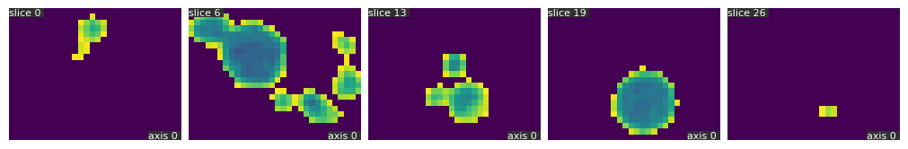
qim3d.viz.plot_connected_components
plot_connected_components(connected_components, component_indexs=None, max_cc_to_plot=32, overlay=None, crop=False, display_figure=True, colormap='viridis', min_value=None, max_value=None, **kwargs)
Plots the connected components from a qim3d.processing.cc.CC object. If an overlay image is provided, the connected component will be masked to the overlay image.
Parameters:
| Name | Type | Description | Default |
|---|---|---|---|
connected_components
|
CC
|
The connected components object. |
required |
component_indexs
|
list or tuple
|
The components to plot. If None the first max_cc_to_plot=32 components will be plotted. Defaults to None. |
None
|
max_cc_to_plot
|
int
|
The maximum number of connected components to plot. Defaults to 32. |
32
|
overlay
|
ndarray or None
|
Overlay image. Defaults to None. |
None
|
crop
|
bool
|
Whether to crop the image to the cc. Defaults to False. |
False
|
display_figure
|
bool
|
Whether to show the figure. Defaults to True. |
True
|
colormap
|
str
|
Specifies the color map for the image. Defaults to "viridis". |
'viridis'
|
min_value
|
float or None
|
Together with vmax define the data range the colormap covers. By default colormap covers the full range. Defaults to None. |
None
|
max_value
|
float or None
|
Together with vmin define the data range the colormap covers. By default colormap covers the full range. Defaults to None |
None
|
**kwargs
|
Any
|
Additional keyword arguments to pass to |
{}
|
Returns:
| Name | Type | Description |
|---|---|---|
figs |
list[Figure]
|
List of figures, if |
Example
import qim3d
vol = qim3d.examples.cement_128x128x128[50:150]
vol_bin = vol < 80
cc = qim3d.segmentation.get_3d_cc(vol_bin)
qim3d.viz.plot_cc(cc, crop=True, display_figure=True, overlay=None, num_slices=5, component_indexs=[4,6,7])
qim3d.viz.plot_cc(cc, crop=True, display_figure=True, overlay=vol, num_slices=5, component_indexs=[4,6,7])
Source code in qim3d/viz/_connected_components.py
9 10 11 12 13 14 15 16 17 18 19 20 21 22 23 24 25 26 27 28 29 30 31 32 33 34 35 36 37 38 39 40 41 42 43 44 45 46 47 48 49 50 51 52 53 54 55 56 57 58 59 60 61 62 63 64 65 66 67 68 69 70 71 72 73 74 75 76 77 78 79 80 81 82 83 84 85 86 87 88 89 90 91 92 93 94 95 96 97 98 99 100 101 102 103 104 105 106 107 108 109 | |
qim3d.viz.plot_metrics
plot_metrics(*metrics, linestyle='-', batch_linestyle='dotted', labels=None, figsize=(16, 6), show=False)
Plots the metrics over epochs and batches.
Parameters:
| Name | Type | Description | Default |
|---|---|---|---|
*metrics
|
tuple[dict[str, float]]
|
Variable-length argument list of dictionary containing the metrics per epochs and per batches. |
()
|
linestyle
|
str
|
The style of the epoch metric line. Defaults to '-'. |
'-'
|
batch_linestyle
|
str
|
The style of the batch metric line. Defaults to 'dotted'. |
'dotted'
|
labels
|
list[str]
|
Labels for the plotted lines. Defaults to None. |
None
|
figsize
|
Tuple[int, int]
|
Figure size (width, height) in inches. Defaults to (16, 6). |
(16, 6)
|
show
|
bool
|
If True, displays the plot. Defaults to False. |
False
|
Returns:
| Name | Type | Description |
|---|---|---|
fig |
Figure
|
plot with metrics. |
Example
train_loss = {'epoch_loss' : [...], 'batch_loss': [...]} val_loss = {'epoch_loss' : [...], 'batch_loss': [...]} plot_metrics(train_loss,val_loss, labels=['Train','Valid.'])
Source code in qim3d/viz/_metrics.py
qim3d.viz.slicer
slicer(volume, slice_axis=0, colormap='magma', min_value=None, max_value=None, image_height=3, image_width=3, display_positions=False, interpolation=None, image_size=None, colorbar=None, mask=None, mask_alpha=0.4, mask_colormap='gray', default_position=0.5, **matplotlib_imshow_kwargs)
Interactive tool to visualize, inspect, and scroll through 2D slices of a 3D volume.
Generates a GUI with a slider to navigate through the dataset along a specified axis. This function is essential for quality control, verifying segmentation masks, or exploring orthogonal views (axial, coronal, sagittal) of a stack.
Key Features:
- Scrollable Interface: Automatically generates a slider for the chosen axis.
- Overlay Support: Visualize segmentation results on top of raw data using the
maskparameter. - Dynamic Contrast: Use
colorbar='slices'to adapt intensity ranges per slice, or'volume'for a global fixed range.
Parameters:
| Name | Type | Description | Default |
|---|---|---|---|
volume
|
ndarray
|
The 3D input data to be sliced. |
required |
slice_axis
|
int
|
The axis to slice along (e.g., 0 for Z, 1 for Y, 2 for X). |
0
|
colormap
|
str or LinearSegmentedColormap
|
Matplotlib colormap name for the volume. |
'magma'
|
min_value
|
float
|
Minimum value for color scaling. If |
None
|
max_value
|
float
|
Maximum value for color scaling. If |
None
|
image_height
|
int
|
Height of the displayed figure. |
3
|
image_width
|
int
|
Width of the displayed figure. |
3
|
display_positions
|
bool
|
If |
False
|
interpolation
|
str
|
Matplotlib interpolation method (e.g., 'nearest', 'bilinear'). |
None
|
image_size
|
int
|
Overrides both |
None
|
colorbar
|
str
|
Strategy for the color bar range.
|
None
|
mask
|
ndarray
|
A 3D segmentation mask to overlay on the volume. |
None
|
mask_alpha
|
float
|
Opacity of the mask overlay (0.0 to 1.0). |
0.4
|
mask_colormap
|
str
|
Matplotlib colormap name for the mask. |
'gray'
|
default_position
|
float or int
|
Initial slice position of the slider.
|
0.5
|
**matplotlib_imshow_kwargs
|
Additional keyword arguments passed to |
{}
|
Returns:
| Name | Type | Description |
|---|---|---|
slicer_obj |
interactive
|
The interactive widget object containing the figure and slider. |
Example
import qim3d

# Load sample data
vol = qim3d.examples.bone_128x128x128

# Visualize with a slider
qim3d.viz.slicer(vol, colormap='bone')
Source code in qim3d/viz/_data_exploration.py
386 387 388 389 390 391 392 393 394 395 396 397 398 399 400 401 402 403 404 405 406 407 408 409 410 411 412 413 414 415 416 417 418 419 420 421 422 423 424 425 426 427 428 429 430 431 432 433 434 435 436 437 438 439 440 441 442 443 444 445 446 447 448 449 450 451 452 453 454 455 456 457 458 459 460 461 462 463 464 465 466 467 468 469 470 471 472 473 474 475 476 477 478 479 480 481 482 483 484 485 486 487 488 489 490 491 492 493 494 495 496 497 498 499 500 501 502 503 504 505 506 507 508 509 510 511 512 513 514 515 516 517 518 519 520 521 522 523 524 525 526 527 528 529 530 531 | |
qim3d.viz.slicer_orthogonal
slicer_orthogonal(volume, colormap='magma', min_value=None, max_value=None, image_height=3, image_width=3, display_positions=False, interpolation=None, image_size=None, colorbar=None, mask=None, mask_alpha=0.4, mask_colormap='gray', default_z=0.5, default_y=0.5, default_x=0.5)
Interactive tool to visualize three orthogonal views (Z, Y, X) side-by-side.
Creates a composite widget displaying Axial, Coronal, and Sagittal slices simultaneously. This is often called a Multi-Planar Reconstruction (MPR) view. It allows users to verify isotropy, check feature continuity across dimensions, or inspect segmentation masks in all three orientations at once.
Key Features:
- Simultaneous Views: Generates three independent sliders for Z, Y, and X axes.
- Linked Settings: Applies colormaps, contrast settings, and masks uniformly across all three views.
- Holistic Inspection: Essential for understanding the 3D structure without rendering a full 3D scene.
Parameters:
| Name | Type | Description | Default |
|---|---|---|---|
volume
|
ndarray
|
The 3D input volume. |
required |
colormap
|
str or LinearSegmentedColormap
|
Matplotlib colormap name. |
'magma'
|
min_value
|
float
|
Minimum value for color scaling. If |
None
|
max_value
|
float
|
Maximum value for color scaling. If |
None
|
image_height
|
int
|
Height of each individual figure in inches. |
3
|
image_width
|
int
|
Width of each individual figure in inches. |
3
|
display_positions
|
bool
|
If |
False
|
interpolation
|
str
|
Matplotlib interpolation method (e.g., 'nearest', 'bilinear'). |
None
|
image_size
|
int
|
Overrides |
None
|
colorbar
|
str
|
Strategy for the color bar range.
|
None
|
mask
|
ndarray
|
A 3D segmentation mask to overlay on all views. |
None
|
mask_alpha
|
float
|
Opacity of the mask overlay (0.0 to 1.0). |
0.4
|
mask_colormap
|
str
|
Matplotlib colormap name for the mask. |
'gray'
|
default_z
|
float or int
|
Initial position for the Z-axis slider (0.0-1.0 relative or exact index). |
0.5
|
default_y
|
float or int
|
Initial position for the Y-axis slider (0.0-1.0 relative or exact index). |
0.5
|
default_x
|
float or int
|
Initial position for the X-axis slider (0.0-1.0 relative or exact index). |
0.5
|
Returns:
| Name | Type | Description |
|---|---|---|
slicer_orthogonal_obj |
HBox
|
A container widget holding the three interactive slicers arranged horizontally. |
Example
import qim3d

# Load sample data
vol = qim3d.examples.fly_150x256x256

# View all three axes side-by-side
qim3d.viz.slicer_orthogonal(vol, colormap="magma")
Source code in qim3d/viz/_data_exploration.py
534 535 536 537 538 539 540 541 542 543 544 545 546 547 548 549 550 551 552 553 554 555 556 557 558 559 560 561 562 563 564 565 566 567 568 569 570 571 572 573 574 575 576 577 578 579 580 581 582 583 584 585 586 587 588 589 590 591 592 593 594 595 596 597 598 599 600 601 602 603 604 605 606 607 608 609 610 611 612 613 614 615 616 617 618 619 620 621 622 623 624 625 626 627 628 629 630 631 632 633 634 635 | |
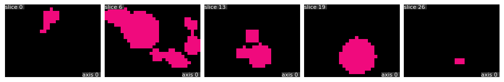
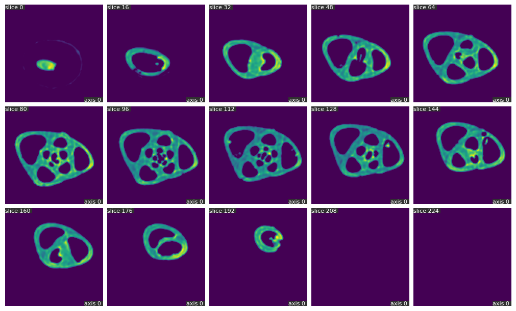
qim3d.viz.slices_grid
slices_grid(volume, slice_axis=0, slice_positions=None, n_slices=15, max_columns=5, colormap='magma', min_value=None, max_value=None, image_size=None, image_height=2, image_width=2, display_figure=False, display_positions=True, interpolation=None, colorbar=False, colorbar_style='small', mask=None, mask_alpha=0.4, mask_colormap='gray', **matplotlib_imshow_kwargs)
Creates a static grid visualization (montage) of multiple 2D slices from a 3D volume.
Generates a mosaic or gallery view of the dataset, ideal for reports, publications, or quick overviews.
Unlike interactive tools, this function produces a static matplotlib figure that can be saved easily.
It supports batch visualization of specific indices, relative positions (e.g., 'mid'), or automatically spaced intervals.
Key Features:
- Flexible Selection: Choose slices by specific index, relative strings ('start', 'mid', 'end'), or automatic linear spacing.
- Publication Ready: Control layout (
max_columns), sizing, and colorbars for export-ready figures. - Mask Overlays: Superimpose segmentation masks directly onto the slice grid.
Parameters:
| Name | Type | Description | Default |
|---|---|---|---|
volume
|
ndarray
|
The 3D input volume to be sliced. |
required |
slice_axis
|
int
|
The axis to slice along (e.g., 0 for Z, 1 for Y, 2 for X). |
0
|
slice_positions
|
int, list[int], str, or None
|
Determines which slices to display.
|
None
|
n_slices
|
int
|
The number of slices to display. Ignored if |
15
|
max_columns
|
int
|
The maximum number of columns in the grid layout. |
5
|
colormap
|
str or LinearSegmentedColormap
|
Matplotlib colormap name. |
'magma'
|
min_value
|
float
|
Minimum value for color scaling. If |
None
|
max_value
|
float
|
Maximum value for color scaling. If |
None
|
image_size
|
int
|
Overrides both |
None
|
image_height
|
int
|
Height of each subplot in inches. |
2
|
image_width
|
int
|
Width of each subplot in inches. |
2
|
display_figure
|
bool
|
If |
False
|
display_positions
|
bool
|
If |
True
|
interpolation
|
str
|
Matplotlib interpolation method (e.g., 'nearest', 'bilinear'). |
None
|
colorbar
|
bool
|
If |
False
|
colorbar_style
|
str
|
Visual style of the colorbar.
|
'small'
|
mask
|
ndarray
|
A 3D segmentation mask to overlay on the slices. |
None
|
mask_alpha
|
float
|
Opacity of the mask overlay (0.0 to 1.0). |
0.4
|
mask_colormap
|
str
|
Matplotlib colormap name for the mask. |
'gray'
|
**matplotlib_imshow_kwargs
|
Additional keyword arguments passed to |
{}
|
Returns:
| Name | Type | Description |
|---|---|---|
fig |
Figure
|
The generated matplotlib figure object containing the grid of slices. |
Raises:
| Type | Description |
|---|---|
ValueError
|
If |
ValueError
|
If |
ValueError
|
If |
Example
import qim3d

# Load sample data
vol = qim3d.examples.shell_225x128x128

# Create a grid of 15 linearly spaced slices
qim3d.viz.slices_grid(vol, n_slices=15)
Source code in qim3d/viz/_data_exploration.py
56 57 58 59 60 61 62 63 64 65 66 67 68 69 70 71 72 73 74 75 76 77 78 79 80 81 82 83 84 85 86 87 88 89 90 91 92 93 94 95 96 97 98 99 100 101 102 103 104 105 106 107 108 109 110 111 112 113 114 115 116 117 118 119 120 121 122 123 124 125 126 127 128 129 130 131 132 133 134 135 136 137 138 139 140 141 142 143 144 145 146 147 148 149 150 151 152 153 154 155 156 157 158 159 160 161 162 163 164 165 166 167 168 169 170 171 172 173 174 175 176 177 178 179 180 181 182 183 184 185 186 187 188 189 190 191 192 193 194 195 196 197 198 199 200 201 202 203 204 205 206 207 208 209 210 211 212 213 214 215 216 217 218 219 220 221 222 223 224 225 226 227 228 229 230 231 232 233 234 235 236 237 238 239 240 241 242 243 244 245 246 247 248 249 250 251 252 253 254 255 256 257 258 259 260 261 262 263 264 265 266 267 268 269 270 271 272 273 274 275 276 277 278 279 280 281 282 283 284 285 286 287 288 289 290 291 292 293 294 295 296 297 298 299 300 301 302 303 304 305 306 307 308 309 310 311 312 313 314 315 316 317 318 319 320 321 322 323 324 325 326 327 328 329 330 331 332 333 334 335 336 337 338 339 340 341 342 343 344 345 346 347 348 349 350 351 352 353 354 355 356 357 358 359 360 361 362 363 364 365 | |
qim3d.viz.threshold
Launches an interactive widget to perform 3D image segmentation via thresholding (binarization).
This tool allows you to explore the volume slice-by-slice to determine the optimal cut-off value for creating a binary mask. It is essential for separating objects of interest from the background based on intensity. The interface provides real-time feedback by displaying the intensity histogram and overlaying the resulting mask on the original data.
Key Features:
- Visualization: Simultaneously views the original slice, intensity histogram, binary mask, and a color overlay.
- Manual Control: Adjust the threshold value precisely using a slider.
- Automatic Algorithms: Applies standard
skimageauto-thresholding methods including Otsu, Isodata, Li, Mean, Minimum, Triangle, and Yen. - Slice Navigation: Scroll through the 3D stack to ensure the chosen threshold works across different depths.
Parameters:
| Name | Type | Description | Default |
|---|---|---|---|
volume
|
ndarray
|
The 3D input data (image stack) to threshold. |
required |
colormap
|
str
|
The Matplotlib colormap for the original image display. |
'magma'
|
min_value
|
float
|
Custom minimum value for display contrast (vmin). If |
None
|
max_value
|
float
|
Custom maximum value for display contrast (vmax). If |
None
|
Returns:
| Name | Type | Description |
|---|---|---|
slicer_obj |
VBox
|
The interactive Jupyter widget containing the visualization plots and control sliders. |
Example
import qim3d

# Load a sample volume
vol = qim3d.examples.bone_128x128x128

# Visualize interactive thresholding
qim3d.viz.threshold(vol)
Source code in qim3d/viz/_data_exploration.py
1614 1615 1616 1617 1618 1619 1620 1621 1622 1623 1624 1625 1626 1627 1628 1629 1630 1631 1632 1633 1634 1635 1636 1637 1638 1639 1640 1641 1642 1643 1644 1645 1646 1647 1648 1649 1650 1651 1652 1653 1654 1655 1656 1657 1658 1659 1660 1661 1662 1663 1664 1665 1666 1667 1668 1669 1670 1671 1672 1673 1674 1675 1676 1677 1678 1679 1680 1681 1682 1683 1684 1685 1686 1687 1688 1689 1690 1691 1692 1693 1694 1695 1696 1697 1698 1699 1700 1701 1702 1703 1704 1705 1706 1707 1708 1709 1710 1711 1712 1713 1714 1715 1716 1717 1718 1719 1720 1721 1722 1723 1724 1725 1726 1727 1728 1729 1730 1731 1732 1733 1734 1735 1736 1737 1738 1739 1740 1741 1742 1743 1744 1745 1746 1747 1748 1749 1750 1751 1752 1753 1754 1755 1756 1757 1758 1759 1760 1761 1762 1763 1764 1765 1766 1767 1768 1769 1770 1771 1772 1773 1774 1775 1776 1777 1778 1779 1780 1781 1782 1783 1784 1785 1786 1787 1788 1789 1790 1791 1792 1793 1794 1795 1796 1797 1798 1799 1800 1801 1802 1803 1804 1805 1806 1807 1808 1809 1810 1811 1812 1813 1814 1815 1816 1817 | |
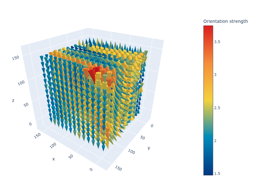
qim3d.viz.vector_field_3d
vector_field_3d(vec, val, select_eigen='smallest', sampling_step=4, max_cones=50000, cone_size=1, verbose=True, colormap='Portland', cmin=None, cmax=None, **kwargs)
Generates an interactive 3D quiver plot (vector field) using cones to visualize local orientation.
This function is designed to visualize the output of structure tensor analysis. It draws 3D cones representing the eigenvectors at various points in the volume. This is widely used to analyze material anisotropy, such as identifying fiber orientations (linear structures) or surface normals (planar structures).
To handle large 3D datasets efficiently, the function downsamples the volume by averaging vectors within grid blocks (sampling_step) and filters to show only the most significant regions (max_cones).
Parameters:
| Name | Type | Description | Default |
|---|---|---|---|
vec
|
ndarray
|
The eigenvectors from the structure tensor. Expected shapes:
|
required |
val
|
ndarray
|
The eigenvalues from the structure tensor, with shape |
required |
select_eigen
|
str
|
Determines which eigenvector to visualize (only used if
|
'smallest'
|
sampling_step
|
int
|
The stride for the sampling grid. A value of |
4
|
max_cones
|
int
|
The maximum number of cones to render. If the sampled grid exceeds this, only the points with the highest eigenvalues (strongest features) are kept. Defaults to 50000. |
50000
|
cone_size
|
float
|
A scaling factor for the size of the cones. Defaults to 1. |
1
|
verbose
|
bool
|
If |
True
|
colormap
|
str
|
The name of the Plotly colorscale. Defaults to 'Portland'. |
'Portland'
|
cmin
|
float
|
The minimum value for the color mapping. If |
None
|
cmax
|
float
|
The maximum value for the color mapping. If |
None
|
**kwargs
|
Additional keyword arguments passed to |
{}
|
Returns:
| Name | Type | Description |
|---|---|---|
fig |
Figure
|
The interactive Plotly figure containing the 3D vector field. |
Raises:
| Type | Description |
|---|---|
ValueError
|
If |
Example
vol = qim3d.examples.fibers_150x150x150
val, vec = qim3d.processing.structure_tensor(vol, smallest = True)
qim3d.viz.vector_field_3d(vec, val, sampling_step=12, max_cones=5000, cone_size = 2)
Notes
Interpreting Eigenvalues and Eigenvectors
The structure tensor yields three eigenvalues (λ₁ ≤ λ₂ ≤ λ₃) and corresponding eigenvectors. The smallest eigenvector (v₁) indicates the predominant orientation, the direction of minimum intensity variation.
| Structure Type | Eigenvalue Pattern | Interpretation |
|---|---|---|
| Linear (fibers, tubes) | λ₁ ≪ λ₂ ≈ λ₃ | Follow v₁ to trace fiber |
| Planar (sheets, boundaries) | λ₁ ≈ λ₂ ≪ λ₃ | v₁ tangent to surface |
| Isotropic (noise, blobs) | λ₁ ≈ λ₂ ≈ λ₃ | No predominant direction |
Source code in qim3d/viz/_structure_tensor.py
330 331 332 333 334 335 336 337 338 339 340 341 342 343 344 345 346 347 348 349 350 351 352 353 354 355 356 357 358 359 360 361 362 363 364 365 366 367 368 369 370 371 372 373 374 375 376 377 378 379 380 381 382 383 384 385 386 387 388 389 390 391 392 393 394 395 396 397 398 399 400 401 402 403 404 405 406 407 408 409 410 411 412 413 414 415 416 417 418 419 420 421 422 423 424 425 426 427 428 429 430 431 432 433 434 435 436 437 438 439 440 441 442 443 444 445 446 447 448 449 450 451 452 453 454 455 456 457 458 459 460 461 462 463 464 465 466 467 468 469 470 471 472 473 474 475 476 477 478 479 480 481 482 483 484 485 486 487 488 489 490 491 492 493 494 495 496 497 498 499 500 501 502 503 504 505 506 507 508 509 510 511 512 513 514 515 516 | |
qim3d.viz.vectors
vectors(volume, vectors, axis=0, volume_colormap='grey', min_value=None, max_value=None, slice_index=None, grid_size=10, interactive=True, figsize=(10, 5), show=False)
Visualizes the local orientation of structures using structure tensor eigenvectors.
This function is designed to analyze anisotropy and fiber direction in 3D volumes. It generates a three-panel visualization to interpret the structure tensor output:
- Quiver Plot: Overlays vector arrows on the image slice to show the dominant direction in the 2D plane.
- Orientation Histogram: displays the distribution of angles, helping to identify if structures are aligned or random.
- Color Map: Renders the slice using an HSV scheme where Hue represents the in-plane angle and Saturation represents the out-of-plane alignment (vectors pointing out of the screen appear desaturated/gray).
Parameters:
| Name | Type | Description | Default |
|---|---|---|---|
volume
|
ndarray
|
The 3D input volume (scalar field). |
required |
vectors
|
ndarray
|
The eigenvectors of the structure tensor, typically shape |
required |
axis
|
int
|
The axis along which to slice the volume for visualization (0, 1, or 2). Defaults to 0. |
0
|
volume_colormap
|
str
|
The colormap for the background volume slice in the quiver plot. Defaults to 'grey'. |
'grey'
|
min_value
|
float
|
Minimum value for the volume display contrast. |
None
|
max_value
|
float
|
Maximum value for the volume display contrast. |
None
|
slice_index
|
int or float
|
The initial slice to display.
|
None
|
grid_size
|
int
|
The spacing between arrows in the quiver plot. Lower values result in denser vector fields. Defaults to 10. |
10
|
interactive
|
bool
|
If |
True
|
figsize
|
tuple[int, int]
|
The width and height of the figure in inches. Defaults to (10, 5). |
(10, 5)
|
show
|
bool
|
If |
False
|
Returns:
| Name | Type | Description |
|---|---|---|
object |
interactive or Figure
|
The visualization object.
|
Raises:
| Type | Description |
|---|---|
ValueError
|
If |
Example
import qim3d

vol = qim3d.examples.NT_128x128x128
val, vec = qim3d.processing.structure_tensor(vol)

# Visualize the structure tensor
qim3d.viz.vectors(vol, vec, axis = 2, interactive = True)
Source code in qim3d/viz/_structure_tensor.py
17 18 19 20 21 22 23 24 25 26 27 28 29 30 31 32 33 34 35 36 37 38 39 40 41 42 43 44 45 46 47 48 49 50 51 52 53 54 55 56 57 58 59 60 61 62 63 64 65 66 67 68 69 70 71 72 73 74 75 76 77 78 79 80 81 82 83 84 85 86 87 88 89 90 91 92 93 94 95 96 97 98 99 100 101 102 103 104 105 106 107 108 109 110 111 112 113 114 115 116 117 118 119 120 121 122 123 124 125 126 127 128 129 130 131 132 133 134 135 136 137 138 139 140 141 142 143 144 145 146 147 148 149 150 151 152 153 154 155 156 157 158 159 160 161 162 163 164 165 166 167 168 169 170 171 172 173 174 175 176 177 178 179 180 181 182 183 184 185 186 187 188 189 190 191 192 193 194 195 196 197 198 199 200 201 202 203 204 205 206 207 208 209 210 211 212 213 214 215 216 217 218 219 220 221 222 223 224 225 226 227 228 229 230 231 232 233 234 235 236 237 238 239 240 241 242 243 244 245 246 247 248 249 250 251 252 253 254 255 256 257 258 259 260 261 262 263 264 265 266 267 268 269 270 271 272 273 274 275 276 277 278 279 280 281 282 283 284 285 286 287 288 289 290 291 292 293 294 295 296 297 298 299 300 301 302 303 304 305 306 307 308 309 310 311 312 313 314 315 316 317 318 319 320 321 322 323 324 325 326 327 | |
qim3d.viz.vol_masked
Applies masking to a volume based on a binary volume mask.
This function takes a volume array volume and a corresponding binary volume mask volume_mask.
It computes the masked volume where pixels outside the mask are set to the background value,
and pixels inside the mask are set to foreground.
Parameters:
| Name | Type | Description | Default |
|---|---|---|---|
volume
|
ndarray
|
The input volume as a NumPy array. |
required |
volume_mask
|
ndarray
|
The binary mask volume as a NumPy array with the same shape as |
required |
viz_delta
|
int
|
Value added to the volume before applying the mask to visualize masked regions. Defaults to 128. |
128
|
Returns:
| Name | Type | Description |
|---|---|---|
ndarray |
ndarray
|
The masked volume with the same shape as |
Source code in qim3d/viz/_metrics.py
qim3d.viz.volumetric
volumetric(volume, aspectmode='data', show=True, save=False, grid_visible=False, colormap='magma', constant_opacity=False, opacity_function=None, min_value=None, max_value=None, samples='auto', max_voxels=256 ** 3, data_type='scaled_float16', camera_mode='orbit', **kwargs)
Renders a 3D volume using high-performance hardware-accelerated ray-casting.
Creates an interactive 3D visualization in the browser using K3D. This function is ideal for inspecting complex voxel data, understanding 3D spatial relationships, or creating exportable HTML representations of a stack. It handles large datasets by automatically downsampling if the size exceeds a set threshold.
Key Features:
- Browser-Based: Renders directly in Jupyter notebooks or exports to standalone HTML.
- Performance: Automatically manages sampling rates and data types (
float16) for smooth interaction. - Customization: Supports custom colormaps, opacity transfer functions, and camera modes.
Parameters:
| Name | Type | Description | Default |
|---|---|---|---|
volume
|
ndarray
|
The 3D input data to be rendered. |
required |
aspectmode
|
str
|
Controls the proportions of the scene axes.
|
'data'
|
show
|
bool
|
If |
True
|
save
|
bool or str
|
Controls saving the output.
|
False
|
grid_visible
|
bool
|
If |
False
|
colormap
|
str, matplotlib.colors.Colormap, or list
|
Colormap for the rendering. Can be a Matplotlib name (e.g., 'magma') or object. |
'magma'
|
constant_opacity
|
bool
|
Deprecated. Use |
False
|
opacity_function
|
str or list
|
Defines the transparency transfer function.
|
None
|
min_value
|
float
|
Minimum value for color scaling. If |
None
|
max_value
|
float
|
Maximum value for color scaling. If |
None
|
samples
|
int or str
|
Number of ray-marching samples.
|
'auto'
|
max_voxels
|
int
|
Maximum number of voxels allowed before downsampling occurs (defaults to approx. 16 million). |
256 ** 3
|
data_type
|
str
|
Internal data type for rendering. |
'scaled_float16'
|
camera_mode
|
str
|
Interaction mode for the camera ( |
'orbit'
|
**kwargs
|
Additional keyword arguments passed to |
{}
|
Returns:
| Name | Type | Description |
|---|---|---|
plot |
Plot
|
The K3D plot object. Returned if |
Raises:
| Type | Description |
|---|---|
ValueError
|
If |
ValueError
|
If |
Tip
The function can be used for object label visualization using a colormap created with qim3d.viz.colormaps.objects along with setting objects=True. The latter ensures appropriate rendering.
Example
Display a volume inline:
Save the rendering to an HTML file without displaying it:
Source code in qim3d/viz/_k3d.py
22 23 24 25 26 27 28 29 30 31 32 33 34 35 36 37 38 39 40 41 42 43 44 45 46 47 48 49 50 51 52 53 54 55 56 57 58 59 60 61 62 63 64 65 66 67 68 69 70 71 72 73 74 75 76 77 78 79 80 81 82 83 84 85 86 87 88 89 90 91 92 93 94 95 96 97 98 99 100 101 102 103 104 105 106 107 108 109 110 111 112 113 114 115 116 117 118 119 120 121 122 123 124 125 126 127 128 129 130 131 132 133 134 135 136 137 138 139 140 141 142 143 144 145 146 147 148 149 150 151 152 153 154 155 156 157 158 159 160 161 162 163 164 165 166 167 168 169 170 171 172 173 174 175 176 177 178 179 180 181 182 183 184 185 186 187 188 189 190 191 192 193 194 195 196 197 198 199 200 201 202 203 204 205 206 207 208 209 210 211 212 213 214 215 | |